Bayesian Learning

Bayesian learning methods provide useful learning algorithms and help us understand other learning algorithms.
The practical learning algorithms are:
- Naive Bayes learning.
- Bayesian belief network learning—combines prior knowledge with observed data.
Bayes reasoning provides the "gold standard" for evaluating other algorithms.

2 Bayes Theorem

Bayes theorem [3] states that \[ P(h\,|\,D) = \frac{P(D\,|\,h) P(h)}{P(D)} \] where
- $P(h)$ = prior probability of hypothesis $h$
- $P(D)$ = prior probability of training data $D$
- $P(h\,|\,D)$ = probability of $h$ given $D$, also known as the posterior probability of $h$.
- $P(D\,|\,h)$ = probability of $D$ given $h$

2.1 Choosing a Hypothesis

Generally want the most probable hypothesis given the training data.
The maximum a posteriori hypothesis is $h_{MAP}$ where \[ \array{ h_{MAP} & = \arg \max_{h \in H} P(h\,|\,D) \\ & = \arg \max_{h \in H} \frac{P(D\,|\,h) P(h)}{P(D)} \\ & = \arg \max_{h \in H}P(D\,|\,h) P(h) } \] we dropped $P(D)$ because its independent of $h$.
If we assume that all hypothesis have the same prior probability, that is $\forall_{i \neq j}P(h_i) = P(h_j)$, then we can simplify even more and choose the maximum likelihood hypothesis \[h_{ML} = \arg \max_{h \in H} P(D\,|\,h) \]

2.2 Example

A patient takes a lab test and the result comes back positive. The test returns a correct positive result in only $98%$ of the cases in which the disease is actually present, and a correct negative result in only $97%$ of the cases in which the disease is not present. Furthermore, $.008$ of the entire population have this cancer. \[ \array{ P(cancer) = .008 & P(\neg cancer) = .992 \\ P(\oplus \,|\, cancer) = .98 & P(\ominus \,|\, cancer) = .02 \\ P(\oplus \,|\, \neg cancer) = .03 & P(\ominus \,|\, \neg cancer) = .97} \]
If a new patient comes in with a positive test result, whats the probability that he has cancer? \[ \array{ P(\oplus\,|\,cancer) P(cancer) = (.98).008 = .0078 \\ P(\oplus\,|\,\neg cancer) P(\neg cancer) = (.03).992 = .0298 } \] so $h_{MAP} = \neg cancer$.

2.3 Probability Formulas

Product rule: probability $P(A \wedge B)$ of a conjunction of two events A and B: \[P(A \wedge B) = P(A\,|\,B) P(B) = P(B\,|\,A) P(A) \]
Sum rule: probability of a disjunction of two events A and B: \[P(A \vee B) = P(A) + P(B) - P(A \wedge B) \]
Theorem of total probability: if events $A_{1}, \ldots, A_{n}$ are mutually exclusive with $\sum_{i = 1}^{n} P(A_{i}) = 1$, then \[P(B) = \sum_{i = 1}^{n} P(B\,|\,A_{i}) P(A_{i})\]

3 Brute Force Bayes Concept Learning

Brute-Force MAP Learning algorithm:
For each hypothesis $h$ in $H$, calculate the posterior probability \[ P(h\,|\,D) = \frac{P(D\,|\,h) P(h)}{P(D)}\] where $D = (d_1\ldots d_m)$ is the set of target values from the set of examples $X = ((x_1,d_1) \cdots (x_m,d_m))$.
Output the hypothesis $h_{MAP}$ with the highest posterior probability \[h_{MAP} = \argmax_{h \in H} P(h\,|\,D)\]
This can be very slow since it applies BT to every $h\in H$.

3.1 Relation to Concept Learning

In concept learning we have an instance space $X$, hypothesis space $H$, training examples $D$. The FindS algorithm finds the most specific hypothesis from $VS_{H,D}$.
Assume fixed set of instances $\langle x_{1}, \ldots, x_{m}\rangle$
Assume $D$ is the set of classifications $D = \langle c(x_{1}), \ldots, c(x_{m})\rangle$
Choose $P(D\,|\,h)$ \[ P(D\,|\,h) = { \{ \array{ 1 & if \forall_{d_i \in D} d_i = h(x_i)\\ 0 & otherwise } } \]
Choose $P(h)$ to be uniform distribution so that $P(h) = \frac{1}{|H|}$ for all $h$ in $H$
Then we can say that \[ P(h\,|\,D) = { \{ \array{ \frac{1}{|VS_{H,D}|} & if h is consistend with D \\ 0 & otherwise. } } \]
What happens in Brute force BCL is that all hypotheses start with with same probability then the inconsistent hypotheses drop to zero while the rest share equally.
Every consistent hypothesis is a MAP hypothesis.

3.2 MAP Hypothesis and Consistent Learners

We showed that, in the given setting, every hypothesis consistent with $D$ is a MAP hypothesis.
Let a consistent learner be one that outputs a hypothesis with zero error over training examples.
Every consistent learner outputs a MAP hypothesis if we assume uniform prior over $H$ and deterministic noise-free examples.
For example, since Find-S outputs a consistent hypothesis, it outputs a MAP hypothesis, all without manipulating probabilities!

4 Learning A Real-Valued Function

Consider any real-valued target function $f$.
Training examples $\langle x_{i}, d_{i} \rangle$, where $d_{i}$ is noisy training value. $d_{i} = f(x_{i}) + e_{i}$, and $e_{i}$ is random variable (noise) drawn independently for each $x_{i}$ according to some Gaussian distribution with mean=0.
The maximum likelihood hypothesis $h_{ML}$ we defined earlier as \[ \array{ h_{ML} &= \argmax_{h \in H} p(D\,|\,h) \\ &= \argmax_{h \in H} \prod_{i=1}^{m} p(d_{i}\,|\,h) } \] if we replace that probability with its equation and simplify we will eventually get \[ h_{ML} = \argmin_{h \in H} \sum_{i=1}^{m} \left(d_{i} - h(x_{i})\right)^{2} \]
Therefore, $h_{ML}$ is the hypothesis that minimizes the sum of the squared errors, if observations are generated by adding Normal noise with zero main to the true data.
Under these conditions any learning algorithm that minimizes the squared error will output a maximum likelihood hypothesis.

5 Learning To Predict Probabilities

Consider predicting survival probability from patient data
Training examples $\langle x_{i}, d_{i} \rangle$, where $d_{i}$ is 1 or 0
Want to train neural network to output a probability given $x_i$ (not a 0 or 1)
In this case can show \[ h_{ML} = \argmax_{h \in H} \sum_{i=1}^{m} d_{i} \ln h(x_{i}) + (1-d_{i}) \ln (1 - h(x_{i})) \] The negation of this quantity is known as the cross entropy.
In order to maximize that we would need to do gradient ascent on it, wrt the edge weight. This weight update works out to be \[ w_{jk} \leftarrow w_{jk} + \Delta w_{jk}\] where \[ \Delta w_{jk} = \eta \sum_{i=1}^{m} (d_{i} - h(x_{i})) x_{ijk} \]
This is the same rule used by Backpropagation except that Backpropagation multiplies by an extra term $h(x_i)(1 - h(x_i))$, which is the derivative of the sigmoid function.
Backpropagation updates seek ML hypothesis under the assumption that training data can be modeled by Normal noise on the target function.
Cross entropy updates seek ML hypothesis under the assumption that observed boolean value is a probabilistic function of input instance.

6 Minimum Description Length Principle

We can interpret the definition of $h_{MAP}$ in terms of the basic concepts of information theory \[ \array{ h_{MAP} &= &\arg \max_{h \in H}P(D\,|\,h) P(h) \\ &= &\arg \max_{h \in H} \log_{2} P(D\,|\,h) + \log_{2} P(h) \\ &= &\arg \min_{h \in H} - \log_{2} P(D\,|\,h) - \log_{2} P(h) } \] This equation can be interpreted as a statement that short hypotheses are preferred!
- $- \log_{2} P(h)$ is length of $h$ under optimal code
- $- \log_{2} P(D\,|\,h)$ is length of $D$ given $h$ under optimal code
The minimum description length principle recomends choosing the hypothesis that minimizes the sum of these two description lengths.
If a representation of hypotheis is chosen so that the size of $h$ is $- \log_2 P(h)$ and if a representation for exceptions is chosen so that the encoding length of $D$ given $h$ is $- \log_2 P(D\,|\,h)$ then the MDL principle produces MAP hypotheses.

7 Bayes Optimal Classifier

So far we've sought the most probable hypothesis given the data $D$ (i.e., $h_{MAP}$)
Given new instance $x$, what is its most probable classification?
$h_{MAP}(x)$ is not the most probable classification!
For example, given three possible hypotheses: \[ P(h_{1}\,|\,D)=.4, P(h_{2}\,|\,D)=.3, P(h_{3}\,|\,D)=.3 \] ($h_1$ is the MAP hypothesis) and given a new instance $x$, \[ h_{1}(x)=\oplus, h_{2}(x)=\ominus, h_{3}(x)=\ominus \] what is the most probable classification of $x$, $\oplus$ or $\ominus$?
The MAP hypothesis ($h_1$) says it is $\oplus$, but if we consider all hypothesis they say that is is $\ominus$ with probability .6. So the most probable classification is $\ominus$.

7.1 Bayes Optimal Classification

Bayes optimal classification \[ \arg \max_{v_{j} \in V} \sum_{h_{i} \in H} P(v_{j}\,|\,h_{i}) P(h_{i}\,|\,D)\]
Example: \[ \array{ P(h_{1}\,|\,D)=.4, & P(\ominus \,|\,h_{1})=0, & P(\oplus \,|\,h_{1})=1 \\ P(h_{2}\,|\,D)=.3, & P(\ominus \,|\,h_{2})=1, & P(\oplus \,|\,h_{2})=0 \\ P(h_{3}\,|\,D)=.3, & P(\ominus \,|\,h_{3})=1, & P(\oplus \,|\,h_{3})=0 } \] therefore \[ \array{ \sum_{h_{i} \in H} P(\oplus \,|\,h_{i}) P(h_{i}\,|\,D) & = & .4 \\ \sum_{h_{i} \in H} P(\ominus \,|\,h_{i}) P(h_{i}\,|\,D) & = & .6 } \] and \[ \array{ \arg \max_{v_{j} \in V} \sum_{h_{i} \in H} P(v_{j}\,|\,h_{i}) P(h_{i}\,|\,D) & = & \ominus }\]

8 Gibbs Algorithm

Bayes optimal classifier provides best result, but can be expensive if many hypotheses.
Gibbs algorithm:
1. Choose one hypothesis at random, according to $P(h\,|\,D)$
2. Use this to classify new instance
Surprising fact: Assume target concepts are drawn at random from $H$ according to priors on $H$. Then: \[ E[error_{Gibbs}] \leq 2 E[error_{Bayes Optimal}] \] So, if the learner correctly assumes a uniform prior distribution over $H$, then
- Pick any hypothesis from VS, with uniform probability
- Its expected error is no worse than twice Bayes optimal

9 Naive Bayes Classifier

The naive bayes classifier is among the set of practical learning methods.
It should be used when
1. There is large set of training examples.
2. The attributes that describe instances are conditionally independent given classification.
It has been used in many applications such as diagnosis and the classification of text documents.

9.1 Naive Bayes Classifier

Assumes all instances $x \in X$ are described by attributes $\langle a_{1}, a_{2} \ldots a_{n} \rangle$.
Assume target function $f: X \rightarrow V$, where $V$ is some finite set.
Most probable value of $f(x)$ given $x = \langle a_{1}, a_{2} \ldots a_{n} \rangle$ is: \[ \array{ v_{MAP} &= &\argmax_{v_{j} \in V} P(v_{j} \,|\, a_{1}, a_{2} \ldots a_{n}) \\ v_{MAP} &= &\argmax_{v_{j} \in V} \frac{P(a_{1}, a_{2} \ldots a_{n}\,|\,v_{j}) P(v_{j})}{P(a_{1}, a_{2} \ldots a_{n})} \\ v_{MAP} &= &\argmax_{v_{j} \in V} P(a_{1}, a_{2} \ldots a_{n}\,|\,v_{j}) P(v_{j}) } \]
Naive Bayes assumes conditional independence given the target value, that is \[ P(a_{1}, a_{2} \ldots a_{n}\,|\,v_{j}) = \prod_{i} P(a_{i} \,|\, v_{j}) \]
Naive Bayes classifier: \[ v_{NB} = \argmax_{v_{j} \in V} P(v_{j}) \prod_{i} P(a_{i} \,|\, v_{j}) \]

9.2 Naive Bayes Algorithm

Naive Bayes Algorithm has a learning and a classifying functions.

Naive_Bayes_Learn(examples)
For each target value $v_j$

$\hat{P}(v_j) \leftarrow $ estimate $P(v_j)$
For each attribute value $a_i$ of each attribute $a$ $\hat{P}(a_i\,|\,v_j) \leftarrow$ estimate $P(a_i\,|\,v_j)$

Classify_New_Instance($x$) \[ v_{NB} = \argmax_{v_{j} \in V} \hat{P}(v_{j}) \prod_{a_i \in x} \hat{P}(a_{i} \,|\, v_{j}) \]

9.3 Naive Bayes Example

We are trying to determine if its time to PlayTennis given that \[\langle Outlook=sunny, Temp=cool, Humid=high, Wind=strong \rangle \]
We want to compute \[ v_{NB} = \argmax_{v_{j} \in V} P(v_{j}) \prod_{i} P(a_{i} \,|\, v_{j}) \]
Given this set of examples we can calculate that \[ P(PlayTennis = yes) = \frac{9}{14} = .64 \] \[ P(PlayTennis = no) = \frac{5}{14} = .36 \] similarly \[P(Wind = strong \,|\, PlayTennis = yes) = \frac{3}{9} = .33 \] \[P(Wind = strong \,|\, PlayTennis = no) = \frac{3}{5} = .6 \] using these and few more similar probabilities we can calculate \[P(yes) \cdot P(Outlook=sunny \,|\, yes)\cdot P(Temperature = cool \,|\, yes)\cdot P(Humidity = high \,|\, yes)\cdot P(Wind = strong \,|\, yes) = .005 \] \[P(no)\cdot P(Outlook=sunny \,|\, no)\cdot P(Temperature = cool \,|\, no)\cdot P(Humidity = high \,|\, no)\cdot P(Wind = strong \,|\, no) = .021 \]
So \[ v_{NB} = no \]

9.4 Naive Bayes Issues

Conditional independence assumption is often violated \[ P(a_{1}, a_{2} \ldots a_{n}\,|\,v_{j}) = \prod_{i} P(a_{i} \,|\, v_{j}) \] but it works surprisingly well anyway.
We don't need estimated posteriors $\hat{P}(v_j\,|\,x)$ to be correct; need only that \[\argmax_{v_{j} \in V} \hat{P}(v_{j}) \prod_{i} \hat{P}(a_{i} \,|\, v_{j}) = \argmax_{v_{j} \in V} P(v_{j}) P(a_{1} \ldots, a_n \,|\, v_{j}) \]
Naive Bayes posteriors often unrealistically close to 1 or 0.
If none of the training instances with target value $v_j$ have attribute value $a_i$ Then \[ \hat{P}(a_i\,|\,v_j) = 0 \text{, and...}\] \[ \hat{P}(v_{j}) \prod_{i} \hat{P}(a_{i} \,|\, v_{j}) = 0 \] Typical solution is Bayesian estimate for $\hat{P}(a_{i} \,|\, v_{j})$ \[ \hat{P}(a_{i} \,|\, v_{j}) \leftarrow \frac{n_{c} + mp}{n + m} \] where
- $n$ is number of training examples for which $v=v_j$,
- $n_c$ number of examples for which $v=v_j$ and $a=a_i$
- $p$ is prior estimate for $\hat{P}(a_{i} \,|\, v_{j})$
- $m$ is weight given to prior (i.e. number of ``virtual'' examples)

10 Learning to Classify Text

Can we learn to classify which news articles are of interest? which web pages are about astronomy?
Naive Bayes is among most effective algorithms
What attributes shall we use to represent text documents??

10.1 Text Attributes

Target concept: IsItInteresting? : Document $\rightarrow \{\oplus,\ominus\}$
Represent each document by vector of words, one attribute per word position in document, where $a_i$ is the $i^{th}$ word in the document. For simplicity $doc \equiv a_1, a_2 \ldots$.
Let $w_k$ be the $k$th word in the English vocabulary.
Use training examples to estimate \[P(\oplus), P(\ominus), P(doc\,|\,\oplus), P(doc\,|\,\ominus)\]
Naive Bayes conditional independence assumption \[ P(doc\,|\,v_j) = \prod_{i=1}^{length(doc)} P(a_i=w_k \,|\, v_j) \] where $P(a_i=w_k\,|\, v_j)$ is probability that word in position $i$ is $w_k$, given $v_j$.
Also, assume that $\forall_{i,m \in \mathcal{N}} P(a_i=w_k\,|\,v_j) = P(a_m=w_k\,|\,v_j)$, i.e., any word any place.

10.2 Learn Naive Bayes Text

Given a set of Examples, and V.

Collect all words and other tokens that occur in Examples.
- $Vocabulary \leftarrow$ all distinct words and other tokens in $Examples$
Calculate the required $P(v_{j})$ and $P(w_{k}\,|\,v_{j})$ probability terms.
- $docs_{j} \leftarrow $ subset of $Examples$ for which the target value is $v_{j}$
- $P(v_{j}) \leftarrow \frac{|docs_{j}|}{|Examples|}$
- $Text_{j} \leftarrow $ a single document created by concatenating all members of $docs_{j}$
- $n \leftarrow$ total number of words in $Text_{j}$ (counting duplicate words multiple times)
- for each word $w_{k}$ in $Vocabulary$
  - $n_{k} \leftarrow$ number of times word $w_{k}$ occurs in $Text_{j}$
  - $P(w_{k}\,|\,v_{j}) \leftarrow \frac{n_{k} + 1}{n + |Vocabulary|}$

10.3 Classify Naive Bayes Text

Given a Doc

$positions \leftarrow$ all word positions in $Doc$ that contain tokens found in $Vocabulary$
Return $v_{NB}$, where \[v_{NB} = \argmax_{v_{j} \in V} P(v_{j}) \prod_{i \in positions}P(a_{i}\,|\,v_{j}) \]

This algorithm was shown to classify Usenet articles into their appropriate newsgroups with 89% accuracy.
A similar approach was proposed by Paul Graham in A Plan for Spam [4]. Several implementations exist such as Spambayes [5].

11 Bayesian Belief Networks

Naive Bayes assumption of conditional independence is too restrictive, but learning is intractable without some such assumptions. Hmmm.....
Bayesian Belief networks describe conditional independence among subsets of variables
They allow combining prior knowledge about (in)dependencies among variables with observed training data
Also known as, Bayes nets.

11.1 Conditional Independence

$X$ is conditionally independent of $Y$ given $Z$ if the probability distribution governing $X$ is independent of the value of $Y$ given the value of $Z$; that is, if \[ \forall_{x_i,y_j,z_k} P(X = x_i \,|\, Y = y_j, Z = z_k) = P(X = x_i \,|\, Z = z_k) \] more compactly, we write \[ P(X \,|\, Y,Z) = P(X \,|\, Z) \]
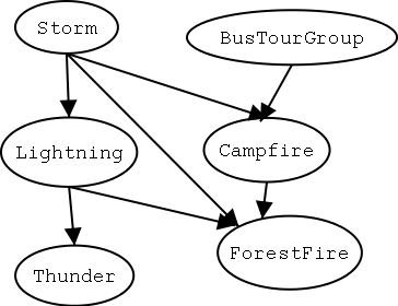
For example, $Thunder$ is conditionally independent of $Rain$, given $Lightning$ \[ P(Thunder \,|\, Rain, Lightning) = P(Thunder \,|\, Lightning) \]
Naive Bayes uses cond. indep. to justify \[ \array{ P(X,Y\,|\,Z) &= & P(X\,|\,Y,Z)\cdot P(Y\,|\,Z) \\ &= & P(X\,|\,Z)\cdot P(Y\,|\,Z) } \]

11.2 Bayesian Belief Network

The network represents a set of conditional independence assertions.
Each node is asserted to be conditionally independent of its nondescendants, given its immediate predecessors.
It forms a directed acyclic graph.
In general, \[P(y_1, \ldots, y_n) = \prod_{i=1}^{n} P(y_i \,|\, Parents(Y_i)) \] where $Parents(Y_i)$ denotes immediate predecessors of $Y_i$ in graph
Joint distribution is fully defined by graph, plus the $P(y_i\,|\,Parents(Y_i))$.

11.3 Inference in Bayesian Networks

How can one infer the (probabilities of) values of one or more network variables, given observed values of others?
Bayes net contains all information needed for this inference.
If there is only one variable with an unknown value then easy to infer it.
In the general case theproblem is NP hard.
In practice, we can succeed in many cases:
Exact inference methods work well for some network structures.
Monte Carlo methods “simulate” the network randomly to calculate approximate solutions.

11.4 Learning Bayesian Networks

Much of the research in Bayesian nets goes into how to use them. We are, instead, interested in learning them.
The network structure might be known or unknown.
Training examples might provide values of all network variables, or just some.
If the structure known and we can observe all variables then its easy as training a Naive Bayes classifier.

11.4.1 Learning Bayesian Networks

Suppose structure known, variables partially observable. For example we observe (ForestFire, Storm, BusTourGroup, Thunder), but not (Lightning, Campfire)
We can use a method similar to training neural network with hidden units.
Specifically, we will use gradient ascent.
We want to converge to network $h$ that (locally) maximizes $P(D\,|\,h)$

11.4.2 Gradient Ascent for Bayes Nets

Let $w_{ijk}$ denote one entry in the conditional probability table for variable $Y_i$ in the network \[ w_{ijk} = P(Y_i=y_{ij}\,|\,Parents(Y_i) = \text{the list} u_{ik} \text{of values}) \] e.g., if $Y_i = Campfire$, then $u_{ik}$ might be $\langle Storm=T, BusTourGroup=F \rangle$
Perform gradient ascent by repeatedly
1. update all $w_{ijk}$ using training data $D$ \[w_{ijk} \leftarrow w_{ijk} + \eta \sum_{d \in D} \frac{P_h(y_{ij}, u_{ik} \,|\, d)}{w_{ijk}} \]
2. then, re-normalize the $w_{ijk}$ to assure $\sum_{j} w_{ijk} = 1$ and $0 \leq w_{ijk} \leq 1$
If some of the probabilities are not present in the data they can be derived via inference from the net.
Again, this only finds locally optimal conditional probabilities.

11.5 The Expectation Maximization Algorithm

The EM algorithm can also be used to learn a Bayes net.

Calculate probabilities of unobserved variables, assuming $h$.
Calculate new $w_{ijk}$ to maximize $E[\ln P(D\,|\,h)]$ where $D$ now includes both observed and (calculated probabilities of) unobserved variables.

When the structure of the network is unknown we can use algorithms that use greedy search to add/subtract edges and nodes. This is an active area of research.

11.5.1 When To Use EM Algorithm

Data is only partially observable.
Unsupervised clustering (target value unobservable).
Supervised learning (some instance attributes unobservable).
Can be used to:
Train Bayesian Belief Networks.
Unsupervised clustering (AUTOCLASS).
Learning Hidden Markov Models.

11.5.2 EM Example: Generating Data from k Gaussians

Imagine the examples are generated by choosing instances $x$ from $k$ Gaussians, with uniform probability.
The learning task is to output a hypothesis that describes the means $\langle \mu_1, \ldots, \mu_k \rangle$ of the $k$ distributions.
We don't know which instance $x_i$ was generated by which Gaussian.
We would like to find a maximum likelihood hypothesis for those means, that is, the maximum likelihood estimates of $\langle \mu_1, \ldots, \mu_k \rangle$.
Think of full description of each instance as $y_i = \langle x_i, z_{i1}, z_{i2} \rangle$, where
1. $z_{ij}$ is 1 if $x_i$ generated by $j$th Gaussian
2. $x_i$ observable
3. $z_{ij}$ unobservable

11.5.3 EM for Estimating k Means

EM Algorithm: Pick random initial $h = \langle \mu_1, \mu_2 \rangle$, then iterate

E step: Calculate the expected value $E[z_{ij}]$ of each hidden variable $z_{ij}$, assuming the current hypothesis $h = \langle \mu_1, \mu_2 \rangle$ holds. \[ \array{ E[z_{ij}] & = & \frac{p(x=x_i \,|\, \mu = \mu_j)}{\sum_{n=1}^{2} p(x = x_i \,|\, \mu=\mu_n)} \\ & = & \frac{e^{-\frac{1}{2 \sigma^2} (x_i - \mu_j)^2}}{\sum_{n=1}^{2} e^{-\frac{1}{2 \sigma^2} (x_i - \mu_n)^2}} } \]
M step: Calculate a new maximum likelihood hypothesis $h' = \langle \mu_1', \mu_2' \rangle$, assuming the value taken on by each hidden variable $z_{ij}$ is its expected value $E[z_{ij}]$ calculated above. Replace $h = \langle \mu_1, \mu_2 \rangle$ by $h' = \langle \mu_1', \mu_2' \rangle$. \[ \mu_j \leftarrow \frac{\sum_{i=1}^m E[z_{ij}] x_i}{\sum_{i=1}^m E[z_{ij}]} \]

11.5.4 EM Algorithm

Converges to local maximum likelihood $h$ and provides estimates of hidden variables $z_{ij}$
In fact, local maximum in $E[\ln P(Y\,|\,h)]$
$Y$ is complete (observable plus unobservable variables) data
Expected value is taken over possible values of unobserved variables in $Y$

11.5.5 General EM Problem

Given:

Observed data $X=\{x_1, \ldots, x_m\}$
Unobserved data $Z=\{z_1, \ldots, z_m\}$
Parameterized probability distribution $P(Y\,|\,h)$, where
1. $Y=\{y_1, \ldots, y_m\}$ is the full data $y_i = x_i \union z_i$ and $h$ are the parameters

Determine:

$h$ that (locally) maximizes $E[\ln P(Y\,|\,h)]$

11.5.6 General EM Method

Define likelihood function $Q(h' \,|\, h)$ which calculates $Y = X \union Z$ using observed $X$ and current parameters $h$ to estimate $Z$ \[ Q(h' \,|\, h) \leftarrow E[ \ln P(Y \,|\, h') \,|\, h, X ] \]

E step: Calculate $Q(h'\,|\,h)$ using the current hypothesis $h$ and the observed data $X$ to estimate the probability distribution over $Y$. \[ Q(h' \,|\, h) \leftarrow E[ \ln P(Y \,|\, h') \,|\, h, X ] \]
M step: Replace hypothesis $h$ by the hypothesis $h'$ that maximizes this $Q$ function. \[ h \leftarrow \argmax_{h'} Q(h' \,|\, h) \]

11.6 Summary of Bayes Nets

Combine prior knowledge with observed data
Impact of prior knowledge (when correct!) is to lower the sample complexity
Active research areas
1. Extend from boolean to real-valued variables
2. Parameterized distributions instead of tables
3. Extend to first-order instead of propositional systems
4. More effective inference methods