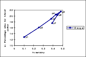
Figure: Scatter plot of volatility versus the percentage of time that the 1-level seller wins (w). The populations are the same as in Figure 3.
In these population sets we explored the advantages that a 1-level seller has over identical 0-level sellers. The advantage was non-existent when all sellers returned the same quality (i.e. when the prices reached an equilibrium), but increased as the sellers started to diverge in the quality they returned. In order to make these findings useful when building agents, we needed a way to make quantitative predictions as to the benefits of keeping 1-level models. It turns out that these benefits can be predicted, not by the population type as we had first guessed, but by the price volatility.

Figure: Scatter plot of volatility versus the percentage of time that
the 1-level seller wins (w). The populations are the same as in
Figure 3.
We define volatility as the number of times the price changes from one auction to the next, divided by the total number of auctions. Figure 4 shows the linear relation between volatility and the percentage of times the 1-level seller wins. The two lines correspond to two ``types'' of volatility. The first line ( p1-p5) is when the buyers' second-favorite (and possibly, the third, fourth, etc) equilibrium price is greater than her most preferred one. In these cases the buyers and sellers fight among the two most preferred prices, the sellers pulling towards the higher equilibrium price, as shown by the two peaks in p4-p5 in Figure 3. The other line correspond to cases where the buyers' preferred equilibrium price is greater than the runner-ups.
The slope of these lines can be easily calculated and the resulting
function can be used by a seller agent for making a quantitative
prediction as to how much he would benefit by switching to 1-level
models. That is, he could measure price volatility, multiply it by the
appropriate slope, and the resulting number would be the percentage of
times he would win. However, for this to work the agent needs to know
that all eight buyers and five sellers are 0-level modelers. Also,
slight changes in our learning parameters ( ![]() and
and ![]() ) lead to slight changes
in the slopes. Still, we hope to eventually generalize this process so
that we can make predictions for all possible combinations (i.e. x
buyers, y sellers) of agents and learning parameters.
) lead to slight changes
in the slopes. Still, we hope to eventually generalize this process so
that we can make predictions for all possible combinations (i.e. x
buyers, y sellers) of agents and learning parameters.
Table 1: Summary of lessons. In all cases the buyers had identical
value and quality assessment functions. Sellers were constrained to
always return the same quality.
We also want to make clear a small caveat, which is that the volatility that is correlated to the usefulness of keeping 1-level models, is the volatility of the system with the agent already doing 1-level modeling. Fortunately, having one agent change from 0-level to 1-level does not have a great effect on the volatility as long as there are enough (i.e. more than five or so) other sellers.
In all populations where the buyers are 0-level, we saw that it really pays for the sellers to have low costs because this allows them to lower their prices to fit almost any demand. Since the buyers have 0-level models, these sellers can also raise their prices when appropriate, in effect ``pretending'' to be the high-quality sellers, and make an even more substantial profit. The buyers are the losers in such situations.
![]()
![]()
![]()
![]()
Next: 1-level buyers and 0
Up: Lessons
Previous: 0-level buyers and sellers.