Illustrating
Probability Propagation in Bayesian Networks using Local Computations
This document describes the algorithms used for probabilistic inference on a Bayesian network. This presentation is based on the text “probabilistic Networks and Expert Systems” by R. G. Cowell, A. P. Dawid, S. L. Lauritzen, and D. J. Spiegelhalter. An example from Finn Jensen’s book “Introduction to Bayesian Networks” is used to illustrate these concepts.
“ . . . The premise underlying the construction of a probabilistic network is that, while the overall problem is too large … for calculating the probabilities, the individual cliques in the triangulated moral graph are of manageable size. In particular, we can perform certain operations, such as marginalization or conditioning, within any clique . . . “
Let a strictly positive joint
probability density for X, Y, Z
factorize as
![]() (1)
(1)
The equation implies[1]
X╨Z|Y and it also suggests a junction tree with two cliques
and one separator:
![]()
We can obtain the marginal
probability density p(x,y) by marginalizing over z
![]() (2)
(2)
Let
![]() (3)
(3)
Then
![]() (4)
(4)
The
equation can be seen as “passing a message XY <- YZ via their separator,”
to obtain p(x,y), where the message is
expressed by h*(y), the separator is
1/h(y), and the update ratio is
h*(y)/h(y).
Note
that
![]() , (5)
, (5)
i.e., f*(x,y) is a marginal of
p(x,y,z)
Using the marginal density f*(x,y),
we can convert into
![]() (6)
(6)
Note that the new equation
expresses p(x,y,z) in terms of message between the two cliques, the marginal
f*(x,y), and g(y,z).
We can also obtain the marginal
density for p(y,z). This would be visualized as “passing a message in the
opposite direction,” i.e.,
XY -> YZ.
This is done by marginalizing
over x the marginal of p(x,y,z) which we obtained in f*(x,y). Intuitively:
![]() (7)
(7)
or opting for the hard approach
![]() (8)
(8)
Parallel to eq. 4 we calculate
![]() (9)
(9)
i.e., we have marginalized
p(x,y,z) over x. With this, we can express p(x,y,z) in terms of the new
messages (compare with eq. 1):
![]() (10)
(10)
“… By the passage of the two
flows (messages) we have transformed the original representation of p(x,y,z)
into a new one involving only marginal densities.“
Example (From
Finn Jensen: An introduction to Bayesian Networks):
Holmes leaves his house. He
observes that his grass is wet (H). Is it due to rain (R)? or has he forgotten
to turn the Sprinkler (S) off?
Later on, as a second
observation, Holmes notes that Mr. Watson grass (W) is also wet. Holmes is
almost certain that it rained.
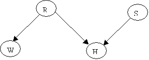
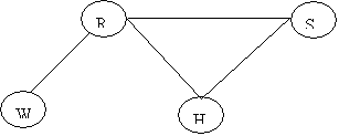
The Junction Tree will be:
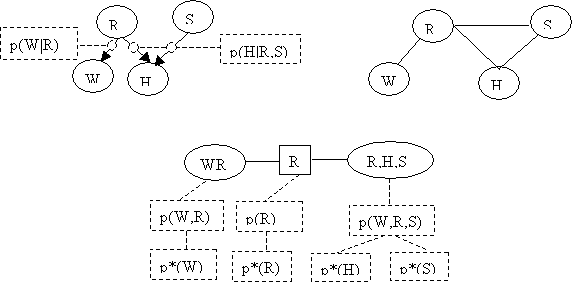
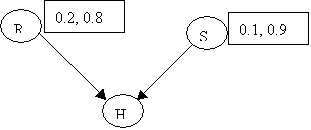
Assume the following priors:
p(R) = (0.2, 0.8) [ y, n ]
p(S) = (0.1, 0.9) [ y, n ]
The conditionals are:
|
|
R=y |
R=n |
|
|
R=y |
R=n |
|
W=y |
1.0 |
0.2 |
|
S=y |
(1, 0) |
(0.9, 0.1) |
|
W=n |
0.0 |
0.8 |
|
S=n |
(1, 0) |
(0, 1.0) |
P(W|R) P(H|R,S)
The vectors in the table
represent (H=y, H=n).
Converting P(H|R,S) into the format we have used:
|
R=y |
R=n |
||
|
|
S=y |
S=n |
S=y |
S=n |
|
H=y |
1.0 |
1.0 |
0.9 |
0.0 |
|
H=n |
0.0 |
0.0 |
0.1 |
1.0 |
From the graph we can obtain the
joint probability for the CLQ(H,R,S)
P(H,R,S) = P(H|R,S)P(R,S)
Since R and S are independent (H
is a collider)
P(H,R,S) = P(H|R,S)P(R)P(S)
We can obtain the prior
probability table for p(H,R,S) using the expression
p(H,R,S)
= p(H|R,S)p(R)p(S)
e.g.,
p(H=y,R=y,S=n) = p(H=y|R=y,S=n)*p(R=y)*p(S=n)
=
1.0*0.2*0.9 = 0.18
p(H=n,R=n,S=n) = 1.0*0.8*0.9 = 0.72
Summarizing in table form:
|
R=y |
R=n |
||
|
|
S=y |
S=n |
S=y |
S=n |
|
H=y |
0.02 |
0.18 |
0.072 |
0.0 |
|
H=n |
0.0 |
0.0 |
0.008 |
0.72 |
We can obtain p(H) by
marginalizing R and S out of P(H,R,S)
|
R=y |
R=n |
|
||
|
|
S=y |
S=n |
S=y |
S=n |
p(H) |
|
H=y |
0.02 |
0.18 |
0.072 |
0.0 |
0.272 |
|
H=n |
0.0 |
0.0 |
0.008 |
0.72 |
0.728 |
P(H) =
(0.272, 0.728)
Doing the same for p(W),
starting off with p(W,R)
p(W,R) =
p(W|R)p(R)
p(W,R) =
p(w=y|r=y)p(R=y)=1.0*0.2 = 0.20
p(W,R) =
p(w=y|r=n)p(R=y)=0.2*0.8 = 0.16
p(W,R) =
p(w=n|r=y)p(R=n)=0.0
p(W,R) =
p(w=n|r=n)p(R=n)=0.8*0.8 = 0.64
|
|
R=y |
R=n |
p(W) |
|
W=y |
0.2 |
0.16 |
0.36 |
|
W=n |
0.0 |
0.64 |
0.64 |
This completes the initialization
phase. The network looks like:
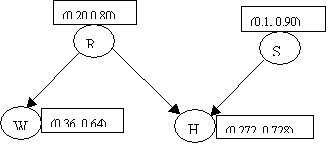
We are ready to receive
evidence.
Suppose we observe that H=y. A
new table p*(H,R,S) is needed.
This table is created by zeroing
the entries for H=n from the table p(H,R,S), and then dividing by p(H=y)
|
R=y |
R=n |
||
|
|
S=y |
S=n |
S=y |
S=n |
|
H=y |
0.02*1/.272 |
0.18*1/.272 |
0.072*1/.272 |
0.0*1/.272 |
|
H=n |
0.0*0.0 |
0.0*0.0 |
0.008*0 |
0.0*0 |
|
R=y |
R=n |
||
|
|
S=y |
S=n |
S=y |
S=n |
|
H=y |
0.074 |
0.662 |
0.264 |
0.00 |
|
H=n |
0.00 |
0.00 |
0.00 |
0.00 |
We marginalize from p*(H,R,S) on
(H,S) and on (H,R) to obtain
p*(R)=
(0.736, 0.264) and p*(S)=(0.339,
0.662).
Now we use the new p*(R) to
update p(W,R), using
p*(W,R)
= p(W|R)*p*(R) = p(W,R)[ p*(R)/p(R) ]
|
|
R=y |
R=n |
|
W=y |
0.2*0.736/0.2 |
0.16*0.264/0.8 |
|
W=n |
0.0 |
0.64*0.264/0.8 |
|
|
R=y |
R=n |
|
W=y |
0.736 |
0.0528 |
|
W=n |
0.0 |
0.2112 |
In summary:
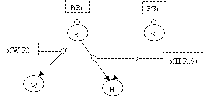


Definitions
A discrete potential on U is a mapping from U. The table of conditional probabilities p(xk|Xpa(k)) forms a potential on kÈpa(k). The potential’s members are real, non-negative numbers, normalized to sum unity for each parent configuration when summed over the states of k.
[Def 1 Extension]
The authors mention two concepts
on this definition: Extension and
projection. Let UÍWÍV. Let f(.) be a potential on U.
That potential is extended to W as follows: Let xÎW. Define f (x)= f (y) where y
is the projection of x onto U.
[Def 2 Multiplication of
Potentials]
Let f and y be two
potentials. The product of the two potentials ![]() is in fact just a dot
product of UÈW.
is in fact just a dot
product of UÈW.
|
|
a1 |
a2 |
a3 |
|
|
c1 |
c2 |
c3 |
|
|
a1 |
a2 |
a3 |
|
B1 |
x1 |
x2 |
x3 |
|
d1 |
p1 |
p2 |
p3 |
|
b1 |
x1p1 |
x2p2 |
x3p3 |
|
B2 |
y1 |
y2 |
y3 |
|
d2 |
q1 |
q2 |
q3 |
|
b2 |
x1q1 |
y2q2 |
y3q3 |
|
B3 |
z1 |
z2 |
z3 |
|
d3 |
r1 |
r2 |
R3 |
|
b3 |
z1r1 |
z2r2 |
z3r3 |
|
|
s |
t |
s*t |
||||||||||
[Def 3 Addition]
Addition is
defined analogously. For potentials f and y on U and W respectively,
we define their sum f and y on U È W by
![]()
Where f and y on the
right hand side have been first extended to U È W.
[Def 4 Division]
Division is
likewise defined in the obvious way, except with special care has to taken when
dividing by zero.
![]() (11)
(11)
[Def 5 Marginalization]
Let WÍUÍV. Let f be a potential on U. The expression ![]() is denoted as the margin,
or sum-margin of f on W,
and it is defined, for x Í W
is denoted as the margin,
or sum-margin of f on W,
and it is defined, for x Í W
![]() (12)
(12)
Where z.x is the element in W
with projections x to U and z to W\U
Section 3 Local Computations on the Junction
Tree
This section describes how to
initialize the tree, compute clique potentials, propagate computations between
adjacent cliques and beyond, and determine when equilibrium is reached.
The section also describes
algorithms for two-phase propagation. All these topics are illustrated with one
example (Child network) at the end of the section.
The graphical representation is
generated from judgments about causal relationships that somehow are expressed
as a chain graph K.
From K a junction
tree T of sets of cliques is generated as described before. The
sets of cliques is denoted C.
The junction tree must be
initialized before it can be used. This provides a localized representation for
the overall distribution.
After initialization, the tree
can receive evidence, which consists of asserting some variables to specific
states. This type of evidence is known
as “hard evidence.”
Local computations are performed
following an orderly sequence that propagates through messages to all the
cliques in the tree.
The density p(.) of the
probability distribution P in the model with a chain graph K and
a set of chain components K factorizes as
 (13)
(13)
and more fully as
 (14)
(14)
A factorization over T of the density of the
joint distribution P on T is constructed. Each clique in C and each separator
in S have potentials denoted as fc and fs . These potentials are
initialized to unity, i.e. each state equals 1.0. For example the potential Y(R,H,S) in the Holmes problem is
|
R=y |
R=n |
||
|
|
S=y |
S=n |
S=y |
S=n |
|
H=y |
1.0 |
1.0 |
1.0 |
1.0 |
|
H=n |
1.0 |
1.0 |
1.0 |
1.0 |
Then each factor in eq. 14 is multiplied into the
potential of any clique that contains all the nodes labeling its arguments.
For example the potential Y(R,H,S) in the Holmes problem becomes, from the
information in the graph, which tells us that
p(H,R,S)
= p(H|R,S)p(R)p(S)
|
R=y |
R=n |
||
|
|
S=y |
S=n |
S=y |
S=n |
|
H=y |
0.02 |
0.18 |
0.072 |
0.0 |
|
H=n |
0.0 |
0.0 |
0.008 |
0.72 |
After each factor has been multiplied we will have
 (15)
(15)
where each separator potential still equals 1.
This representation is called the initial
representation of P, and its potentials are called the initial
potentials.
In order to understand the flow between adjacent cliques
we need to define the following:
[Def 6 Charge]
A collection of non-negative potential functions ![]() is termed as a charge.
is termed as a charge.
[Def 7 Contraction]
For any charge that is defined as a set of non-negative
potential functions ![]() , the right-hand side of the Eq. 15 defines its contraction.
, the right-hand side of the Eq. 15 defines its contraction.
[Def 8 Generalized Potential]
Whenever Eq. 15 holds we call ![]() as a generalized
potential representation of the joint distribution P on a junction
tree T.
as a generalized
potential representation of the joint distribution P on a junction
tree T.
Flow Between Adjacent Cliques
The algorithm is best described as a series of messages between
adjacent cliques and their separators. Each message acts on a clique and its
separator.
Let C1 and C2 be two adjacent
cliques in T, and let S0 be their separator. A message
(or flow) called sum-flow is described, between a source
clique and a sink clique.
Assume a charge F exists, ![]() . The effect of the
message will be to replace this charge by a new one, denoted
. The effect of the
message will be to replace this charge by a new one, denoted ![]() .
.
The new potentials for the sink and the separator are given by eqs. 16, 17. Note that only the sink C2 and the separator S0 are affected by the message.
![]()
![]() (16)
(16)
where lso is
called the update ratio, given by
![]() (17)
(17)
A charge is unaffected by the message if the charge is sum-consistent,
a condition which is defined as
![]() (18)
(18)
Active Flows
Proposition 1: Co is a leaf. To is the
subtree that resulted from separating Co from T1

By induction, for a larger tree (no separators shown, nodes are cliques)
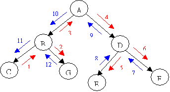
Reaching Equilibrium
See the preliminary definitions in the section. A subtree T’
is live at a stage of a schedule if it has already received active
messages from all its neighbors.
Theorem 1: Suppose we start with a
representation F0 for a
function f that factorizes T and progressively
modify it by following a schedule of messages.
Then whenever T’ is live, its potential is the sum-margin fu’
of f on U’.
Corollary 1: Whenever a clique C is live, its potential is fc.
Corollary 2: Any time after active messages
pass in both directions across an edge of T. the potential for
its separator S is fs.
Corollary 3: Any time after active messages
pass in both directions across an edge of T between cliques C1,
C2, with separator S, the tree becomes sum-consistent with S,
a condition defined as
![]() (19)
(19)
Corollary 4: After passage of a full
schedule of messages, the resulting charge is the marginal charge Ff of f, and the
tree will be sum-consistent, which means that it has reached
equilibrium.
Corollary 5: Suppose that some function f
factorizes on T. Then Ff (charge of f) is
a representation for f, hence,
 (20)
(20)
Section 4 Scheduling the Messages
Inactive messages are not scheduled. There are several
scheduling schemes that can be used to propagate evidence on the junction tree,
all of which should produce the same results.
The main difference is the efficiency of the algorithms.
A popular scheduling scheme, due to Finn Jensen et al.,
is known as the two-phase propagation. An arbitrary clique is
selected to become the root clique. A collection
phase passes messages along the edges directed towards the root clique. The
next phase, called distribution,
passes messages back to the periphery starting at the root.
If A is the root:

Two-Phase Propagation
This scheduling scheme is due to Finn Jensen et al., from Aalborg University in Denmark.
The algorithm schedules the messages in two phases, called collection phase and distribution phase.
The specific actions taken at each phase are:
[Def 9 Collect Evidence]
This is a recursive definition. Note the distinction between calling a message and sending a message. When CE is called in a clique U from neighbor W, U passes the call to all its neighbors except W. After all neighbors have responded to the call with a flow of their own back to U, U passes a flow back to W.

At this point the root clique has absorbed all the available information from all its neighbors. This information must be distributed in a procedure called distribute evidence, described in
[Def 10 Distribute Evidence]
When DE is called for clique U from W, a message (flow) is passed from W to U, and then U propagates the message to its neighbors
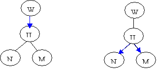
Entering and Propagating Evidence
When evidence e(x) arrives to the network, it enters via the initialized junction tree. A potential containing the node associated to the new evidence is multiplied by [eq 6.19].
The new set of potentials now represents:
![]()
The tree will not reach equilibrium until a full schedule of messages is passed amongst the cliques in both directions.
Once that is done, posterior probabilities can be found by normalizing the potentials to sum to 1, see eqs 6.20, 6.21.
A Propagation Example
This example uses a portion of a child network from the book Cowell et.al. The conditional probabilities involved, p(n4|n2) and p(n15|n4) are shown in Table 3.1, pp. 30 of that book. The tables are
|
|
N4: LHV? |
|
|
N2 Disease? |
Yes |
No |
|
PFC |
0.10 |
0.90 |
|
TGA |
0.10 |
0.90 |
|
Fallot |
0.10 |
0.90 |
|
PAIVS |
0.90 |
0.10 |
|
TAPVD |
0.05 |
0.95 |
|
Lung |
0.10 |
0.90 |
|
|
N15: LHV Report? |
|
|
N4 LHV? |
Yes |
No |
|
|
|
|
|
Yes |
0.90 |
0.10 |
|
NO |
0.05 |
0.95 |
The three nodes form a charge given by
![]()
The initial tables in the cliques are given by p(n4|n2) and p(n15|n4). Initially all the items in the separator are set to unity. Note that the charge is at equilibrium.
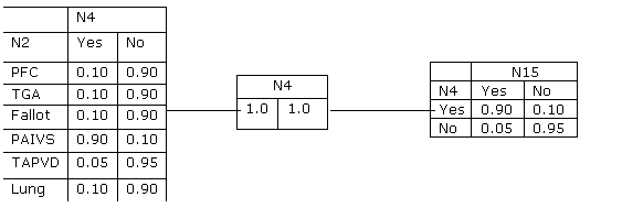
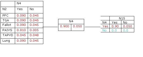
1. Evidence Yes is entered in N15, i.e., i(n15) =(1.0, 0.0).
2. Y*(C14)=p*(n15,n4)=i(n15)´p(n15|n4)={[0.9,0.05],[0.0,0.0]}
3. ![]()
4. The
update ratio is ![]()
5. Y*(C13)=p*(n4,n2)=p*(n4)´ls, resulting in table at left, below:
6. The propagation continues on to the parent(s) of n15 and into the rest of the junction tree. Somehow the propagation comes back into the clique C13. At this point the potential in C13 is that of table 6.1c, reproduced here, at the left:
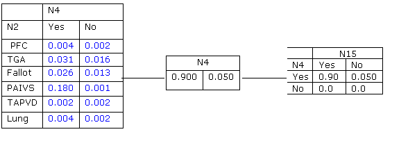
7. The
new separator is calculated by marginalizing n2 out of C13: ![]()
8. The new update ratio is l = ({0.248/0.9}, {0.036/0.05} )= (0.276,0.720). The new potential at C14 is propagated from n4, (0.248, 0.036).
9. Summing all the items of any potential gives us the normalization constant a= 0.284. Dividing each of the elements in all tables by a gives the entries in the table which is the final answer.