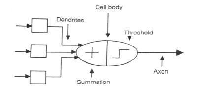
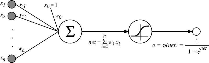
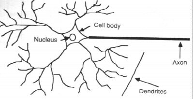
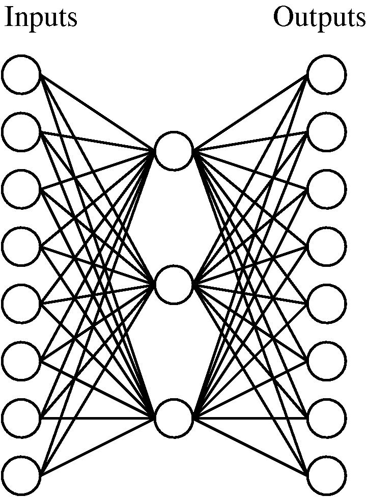
Artificial Neural Networks

Artificial Neural Networks are a robust method for approximating real-valued, discrete-valued, and vector-valued target functions.
They are most effective when used against real-world sensor data.
They stem from a biological metaphor.

1.1 The Human Brain

A neuron

Has about $10^{11}$ neurons each connected to $10^{4}$ other neurons.
Each neuron has inputs which are called dendrites and one output which is called the axon.
The switching time is about $. 001$ second.
It takes around $. 1$ second for the brain to recognize an image, which implies about 100 inference steps.
So, the brain must do some parallel processing on highly distributed data.
ANNs are not identical to human neurons. They are merely simplistic approximations.

1.2 Neural Network Representation

Artificial neuron

An ANN simulates the switching abilities of the neuron body.
ANNs use many of these threshold switching units.
The connections between neurons are weighted.
The desired input is wired to some of the input lines, and so is the output.
The job of the learning algorithm is to properly adjust the weights so the output that results matches the example.
Our goal is to produce a good learning algorithm, not to simulate the brain.

2 When to Use Neural Networks

Input is high-dimensional discrete or real-valued (e.g. raw sensor input)
Output is discrete or real valued
Output is a vector of values
Possibly noisy data
Form of target function is unknown
Human readability of result is unimportant

2.1 ALVINN

The Autonomous Land Vehicle In a Neural Network (ALVINN [3]) is a perception system which learns to control the NAVLAB vehicles by watching a person drive
One of the first examples that neural-networks could do "real-work". It can drive 70mph on highways.
ALVINN's architecture consists of a single hidden layer back-propagation network.
The input layer of the network is a 30x32 unit two dimensional "retina" which receives input from the vehicles video camera.
Each input unit is fully connected to a layer of five hidden units which are in turn fully connected to a layer of 30 output units. The output layer is a linear representation of the direction the vehicle should travel in order to keep the vehicle on the road.

3 Perceptrons

A perceptron takes a vector of real-valued inputs, calculates a linear combination of these, and outputs a 1 if its greater than some threshold or -1 otherwise. Formally, $o (x_{1}, \dots, x_{n}) = {\begin{matrix} 1 & if w_{0} + w_{1} x_{1} + \cdot \cdot \cdot + w_{n} x_{n} > 0 \\ - 1 & otherwise. \end{matrix}$
Sometimes we'll use simpler vector notation $o (\overset{⇀}{x}) = {\begin{matrix} 1 & if \overset{⇀}{w} \cdot \overset{⇀}{x} > 0 \\ - 1 & otherwise. \end{matrix}$ where we assume an additional constant input $x_{0} = 1$ .
Learning involves choosing values for $w_{0}, \dots, w_{n}$ such that the output $o$ value matches the target value $t$ .

3.1 Representational Power of Perceptrons

Decision surface of two-input ( $x_{1}$ and $x_{2}$ ) perceptron.

We can view the perceptron as representing a hyperplane decision surface in n-dimensional space of instances.
Test: Which weights represent $g (x_{1}, x_{2}) = AND (x_{1}, x_{2})$ ? $w_{0} = - . 8, w_{1} = w_{2} = . 5$ which is the line $y = \frac{8}{5} - x$ .
Notice that example (b) is not linearly separable. It is an XOR.
Perceptrons cannot represent XOR, so we will need networks of them.

3.2 Perceptron Training

One way to learn the weights is to start with random weights then apply it to each example, changing the weights to fit.
The perceptron training rule is used to change the weights each time. It does $w_{i} \leftarrow w_{i} + Δ w_{i}$ where $Δ w_{i} = η (t - o) x_{i}$ and $t = c (\overset{⇀}{x})$ is target value, $o$ is perceptron output, and $η$ is small constant (e.g., .1) called learning rate.

3.3 Perceptron Training Rule Convergence

It can be proven that this procedure will converge in finite time if
1. the training examples are linearly separable and
2. the learning rate $η$ is sufficiently small.
If the data are not linearly separable then convergence is not assured.

3.4 Gradient Descent

The delta rule is designed to converge if the examples are not linearly separable.
It does a gradient descent on the hypothesis space.
Consider a simpler linear unit, where $o = w_{0} + w_{1} x_{1} + \cdot \cdot \cdot + w_{n} x_{n}$ Let's learn $w_{i}$ 's that minimize the squared error $E (\overset{⇀}{w}) \equiv \frac{1}{2} \sum_{d \in D} (t_{d} - o_{d})^{2}$ Where $D$ is set of training examples
Lets try to minimize the error.

3.4.1 Gradient Descent Landscape

Gradient $\nabla E [\overset{⇀}{w}] \equiv [\frac{\partial E}{\partial w_{0}}, \frac{\partial E}{\partial w_{1}}, \cdot \cdot \cdot \frac{\partial E}{\partial w_{n}}]$ Training rule: $Δ \overset{⇀}{w} = - η \nabla E [\overset{⇀}{w}]$ i.e., $Δ w_{i} = - η \frac{\partial E}{\partial w_{i}}$
The gradient specifies the direction that produces the steepest increase in $E$ (so, negate it).

3.4.2 Calculating the Gradient Descent

We can calculate the actual value of the gradient descent by differentiating $E$ : $\begin{matrix} \frac{\partial E}{\partial w_{i}} & = & \frac{\partial}{\partial w_{i}} \frac{1}{2} \sum_{d} (t_{d} - o_{d})^{2} \\ = & \frac{1}{2} \sum_{d} \frac{\partial}{\partial w_{i}} (t_{d} - o_{d})^{2} \\ = & \frac{1}{2} \sum_{d} 2 (t_{d} - o_{d}) \frac{\partial}{\partial w_{i}} (t_{d} - o_{d}) \\ = & \sum_{d} (t_{d} - o_{d}) \frac{\partial}{\partial w_{i}} (t_{d} - \overset{⇀}{w} \cdot \overset{⇀}{x_{d}}) \\ \frac{\partial E}{\partial w_{i}} & = & \sum_{d} (t_{d} - o_{d}) (- x_{i, d}) \end{matrix}$
So the weight update (training) rule is $Δ \overset{⇀}{w} = - η \sum_{d \in D} (t_{d} - o_{d}) x_{id}$ where $x_{id}$ is the single input component $x_{i}$ for example $d$ .

3.4.3 Gradient Descent Algorithm

Gradient-Descent(training-examples, η )
- Each training example is a pair of the form $⟨ \overset{⇀}{x}, t ⟩$ , where $\overset{⇀}{x}$ is the vector of input values, and $t$ is the target output value. $η$ is the learning rate (e.g., .05).
Initialize each $w_{i}$ to some small random value
Until the termination condition is met, Do
1. Initialize each $Δ w_{i}$ to zero.
2. For each ⟨ x ⇀,t⟩ in training-examples, Do
  1. Input the instance $\overset{⇀}{x}$ to the unit and compute the output $o$
  2. For each linear unit weight $w_{i}$ , Do $Δ w_{i} \leftarrow Δ w_{i} + η (t - o) x_{i}$
3. For each linear unit weight $w_{i}$ , Do $w_{i} \leftarrow w_{i} + Δ w_{i}$

3.5 Perceptron Learning Summary, so far

Perceptron training rule is guaranteed to succeed if the training examples are linearly separable and the learning rate is sufficiently small.
The linear unit training rule (gradient descent) will converge to the hypothesis with minimum squared error given a sufficiently small learning rate, even with noise and when training data not separable by $H$ .
Gradient descent has two problems
1. Convergence to a local minimum can sometimes be slow.
2. There is no guarantee that we will find the global minimum.

3.6 Incremental (Stochastic) Gradient Descent

The stochastic gradient descent algorithm is a simple variation on gradient descent: instead of adding up the gradients over all examples, we update weights incrementally.
That is, change the weights after each example.
For each training example $d$ in $D$ we compute the gradient $\nabla E_{d} [\overset{⇀}{w}]$ and then $\overset{⇀}{w} \leftarrow \overset{⇀}{w} - η \nabla E_{d} [\overset{⇀}{w}]$
We can view this as going down one of the different landscapes (one for each $d$ ) defined as $E_{d} [\overset{⇀}{w}] \equiv \frac{1}{2} (t_{d} - o_{d})^{2}$ at each step.

3.6.1 Stochastic versus Batch Gradient Descent

Incremental Gradient Descent can approximate Batch Gradient Descent arbitrarily closely if $η$ made small enough.
In stochastic the weights are updated after examining each example.
Batch gradient takes longer in its inner loop (large sum) but it can use a larger step size because of this sum.
Stochastic can often avoid falling into local minima.
NOTE: altough these methods assume unthresholded linear units, they can be easily modified to work on regular perceptrons.

4 Multilayer Networks

In order to represent non-linearly separable functions we need at least two layers of perceptrons.
These networks allow complex classification patterns.
Once we have these complex networks, we need a new algorithm to train them.
Perceptrons are discontinous so they can't be differentiated. This makes it hard to work with.

4.1 Sigmoid Unit

We let $σ (net)$ be the sigmoid function where $σ (net) = \frac{1}{1 + e^{- net}}$ and $net$ is the sum of the weighted inputs, or $net = \sum_{i = 1}^{n} w_{i} x_{i}$
It has the nice property that $\frac{d σ (x)}{dx} = σ (x) (1 - σ (x))$ .
So, we can use it to derive gradient descent rules for the training of multilayer networks.

4.2 Error Gradient for Sigmoid Unit

Since the networks have multiple output units we must redefine $E$ to sum the errors $E (\overset{⇀}{w}) \equiv \frac{1}{2} \sum d \in D \sum_{k \in outputs} (t_{kd} - o_{kd})^{2}$ where $t_{kd}$ and $o_{kd}$ are the target and output values associate with the kth output unit and example $d$ .
After some algebra (not shown) we can derive that the error slope for each weight is $\frac{\partial E}{\partial w_{i}} = - \sum_{d \in D} (t_{d} - o_{d}) o_{d} (1 - o_{d}) x_{i, d}$

4.3 Backpropagation

Initialize all weights to small random numbers.
For each training example Do
1. Input the training example to the network and compute the network outputs
2. For each output unit $k$ calculate its error term $δ_{k}$ $δ_{k} \leftarrow o_{k} (1 - o_{k}) (t_{k} - o_{k})$
3. For each hidden unit $h$ calculate its error term $δ_{h}$ $δ_{h} \leftarrow o_{h} (1 - o_{h}) \sum_{k \in outputs} w_{h, k} δ_{k}$
4. Update each network weight $w_{i, j}$ $w_{i, j} \leftarrow w_{i, j} + Δ w_{i, j}$ where $Δ w_{i, j} = η δ_{j} x_{i, j}$
Goto 2 if termination condition is not met.

4.3.1 Backpropagation Details

It does a gradient descent over the entire network weight vector.
It can be generalized to handle arbitraty directed graphs.
It will find a local min, which might not be the global min. In practice, this has not been a large problem (local min are good enough and large dimension means more escape routes).
A popular technique is to add momemtum $α$ $Δ w_{i, j} (n) = η δ_{j} x_{i, j} + α Δ w_{i, j} (n - 1)$
As always, it minimizes the error over the training examples. Will it generalize?
It can be very slow to train.
But, once trained, it can make new categorizations very fast.
Inductive Bias: is very hard to quantify, but can be characterized as smooth interpolation between data points.

4.3.2 Hidden Layer Representation

Input	H1	H2	H3	Output
10000000	.89	.04	.08	10000000
01000000	.15	.99	.99	01000000
00100000	.01	.97	.27	00100000
00010000	.99	.97	.71	00010000
00001000	.03	.05	.02	00001000
00000100	.01	.11	.88	00000100
00000010	.80	.01	.98	00000010
00000001	.60	.94	.01	00000001

Given this network, can this data set be learned? Results from an actual run tell us so.
The hidden unit encoding resembles a binary encoding.

4.3.3 8-3-8 Plots

Hidden unit encoding

Weights from inputs to a hidden unit

Sum of squared errors

The units converge at different times but the curves look the same.
We can see how one of the hidden units starts to converge to one value then ends up converging to a different one.
In general the weights see little change at first, then a lot of change, then they settle down.

4.3.4 Backpropagation Convergence

Backpropagation does a gradient descent, so it will converge to a local minimum (perhaps not global). To alliviate this you can

add momentum, as before,
use stochastic gradient descent,
train multiple nets with different initial weights.

As we saw in the pictures, convergence is slow at first then fast.

4.4 Representational Power of ANNs

Every boolean function can be represented by network with single hidden layer but might require exponential (in number of inputs) hidden units
Every bounded continuous function can be approximated with arbitrarily small error, by network with one hidden layer.
Any function can be approximated to arbitrary accuracy by a network with two hidden layers.

4.5 Overfitting ANNs

The error decreases monotonically over time as a function of the training set.
But, when measure against the validation set the function is non-monotonic. This line is said to measure the generalization accuracy of the network.
The second figure shows that it is hard to pick the min (the validation curve can have local minima).
Some techniques used to fight overfitting include

Decrease each weight by some small factor during each iteration (weight decay). Keep them small so as to bias against learning complex surfaces.
Provide a validation set and use it to monitor the error. But, be careful not to find a minimum too early.
With small data sets, use k-fold cross-validation: divide pile into k disjoint sets. Each time one of the sets is the validation and the other k-1 are the training data.

5 Face Recognition Example

left

straight

right

Dark is negative and light is positive.
Its a 960-3-4 network.
The first block in the output units is the threshold, the rest represent inputs from the hidden units.
The third line shows the weights from the inputs to the hidden units.
The code and data [4] for this example are available.

6 Alternative Error Functions

Penalize large weights: $E (\overset{⇀}{w}) \equiv \frac{1}{2} \sum_{d \in D} \sum_{k \in outputs} (t_{kd} - o_{kd})^{2} + γ \sum_{i, j} w_{ji}^{2}$
Add a term for errors in the slope of the target function $E (\overset{⇀}{w}) \equiv \frac{1}{2} \sum_{d \in D} \sum_{k \in outputs} [(t_{kd} - o_{kd})^{2} + μ \sum_{j \in inputs} {(\frac{\partial t_{kd}}{\partial x_{d}^{j}} - \frac{\partial o_{kd}}{\partial x_{d}^{j}})}^{2}]$
Tie together weights: e.g., in phoneme recognition network

7 Recurrent Networks

Apply a to time series data.
Use output of network unites at time t as input to units at time t+1.
They need a new training algorithm. Several have been proposed.
A common method of training is to use a simple variation on backpropagation.
This method involves "unfolding" the network over time (as seen in (c)) and then using then applying backpropagation to the new network.

8 Dynamically Modifying Network Structure

Begin with a network with no hidden units then grow as needed by adding new one until the error is reduced. For example, the Cascade-Correlation algorithm.
- It is easy to overfit the data.
Begin with a complex network and prune it as we find unessential connections.
- Weight is almost 0.
- Consider way in which a small variation in the weight affects the Error. More successful method.
In general, they show mixed success in accuracy but can improve training times.

9 Summary

ANNs provide a method for learning real-valued and vector-valued over continuous and discrete-valued attributes.
Backpropagation is the most common algorithm, it works.
The hypothesis space consists of all the functions that can be represented by the network. For three layers this means all function (in some cases an excessive number of nodes might be needed).
Backpropagation uses gradient-descent and so converges to a local minimum.
The hidden layers can invent new features.
Over-fitting is common. It results in networks that generalize poorly