Implementation of Pursuit Task

The original algorithm has been implemented in a simulation of the pursuit task, using the MICE system [12]. The experiments showed some promising results. The overall performance of the agents was maintained while the total number of expanded nodes was reduced by an order of magnitude.

Method Avg. Nodes Avg. Time to

Expanded Capture/Surround

BFS 1 Level 1 /Never Captured

BFS 2 Levels 4 23.4

BFS 3 Levels 13 22.4

BFS 4 Levels 40 17.3

LR RMM 4.2 18.5

Greedy NA 41.97

Table 1: Results of implementation of the Pursuit problem using simple BFS to various levels (i.e. regular RMM), using our Limited Rationality Recursive Modeling algorithm, and using a simple greedy algorithm, in which each predator simply tries to minimize its distance to the prey.

**Table 1:** Results of implementation of the Pursuit problem using simple BFS to various levels (i.e. regular RMM), using our Limited Rationality Recursive Modeling algorithm, and using a simple greedy algorithm, in which each predator simply tries to minimize its distance to the prey.
Method	Avg. Nodes	Avg. Time to
	Expanded	Capture/Surround
BFS 1 Level	1	/Never Captured
BFS 2 Levels	4	23.4
BFS 3 Levels	13	22.4
BFS 4 Levels	40	17.3
LR RMM	4.2	18.5
Greedy	NA	41.97

We designed a function that takes as input a physical situation and a predator in that situation and returns the payoff matrix that the predator expects to get given each of the possible moves they all take. This function is used by all the predators (that is, we assumed all predators were of the same type). A predator's payoff is the sum of two values. The first value is the change in the distance from the predator to the prey between the current situation and the new situation created after all agents have made their moves. The second value is , where k is the number of quadrants around the prey that have a predator in them in the new situation. The quadrants are defined by drawing two diagonal lines across the prey [5, 11].

Since the matrices take into account all possible combinations of moves (5 for each predator and 4 for the prey), they are five-dimensional with a total of 2500 payoff entries. With matrices this big, even in a simple problem, it is easy to see why we wish to minimize the number of matrices we need to generate. We defined the physical situation which the predator is in as its relative position to the prey and to the other predators. These situations were then generalized such that distances greater than two are indistinguishable, except for quadrant information. This generalization formula served to shrink the number of buckets or keys in our hash table to a manageable number (from to around 3000). Notice also that the number of buckets remains constant no matter how big the grid is.

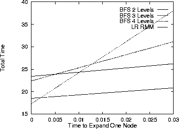
Figure 6: Plot of the total time that would, on average, be spent by the agents before capturing the prey, for each method. The x axis represents the amount of time it takes to expand a node as a percentage (more or less) of the time it takes the agent to take action.