Reinforcement Learning

This talk is based on

Tom M. Mitchell. Machine Learning. [1] McGraw Hill. 1997. Chapter 13.
and his slides [2].
An excellent resource is Reinforcement Learning: An Introduction [3] by Sutton and Barto (free!).

1 Introduction

So far, our machine learning problems have assumed:
1. that we can present the learner with correct examples,
2. and that learning goes first, then we test.
Imagine a robot learning to dock with the batter charger.
It gets a reward (charge) when successful, but must determine how to encourage actions that led there (temporal credit assignment problem).
- The reward might be probabilistic.
It can explore the domain, finding a better route? (exploration vs. exploitation problem)
The state might only be partially observable.
It might have to learn several related task with the same environment and using the same sensors.

1.1 TD-Gammon

The TD-Gammon [4] system learned to play championship Backgammon by playing 1.5 million games against itself.
It received an immediate reward for +100 for a win, -100 for a loss.
Equal to the best human.

1.2 Reinforcement Learning Problem

The agent is in a state $s_0$, takes action $a_0$ for which it receives a reward of $r_0$ and ends up at $s_1$: \[ s_0 \rightarrow^{r_0} s_1 \rightarrow^{r_1} s_2 \rightarrow^{r_2} s_3 \cdots \]
We define the problem:
$S$ finite set of states
$A$ finite set of actions
$r_t = r(s_t,a_t)$
$s_{t+1} = \delta(s_t,a_t)$
We also assume that $s_{t+1}$ and $r_t$ depend only on the current state and action.
That is, the system is a Markov Decision Process.
Note that $\delta$ and $r$ might be nondeterministic.
Also, the agent might not know $\delta$ and $r$

1.3 The Learning Task

Given that the agent inhabits a Markov process it must now learn action policy $\pi : S \rightarrow A$ that maximizes \[ E[r_t + \gamma r_{t+1} + \gamma^2 r_{t+2} + \ldots ] \] from any starting state in $S$.
$0 \leq \gamma < 1$ is the discount factor for future rewards.
The target function is $\pi: S \rightarrow A$.
The training examples are of the form $\langle \langle s, a \rangle , r \rangle$

1.4 Value function

For each possible policy $\pi$ the agent might adopt, we can define an evaluation function over states \[ V^{\pi}(s) \equiv r_{t} + \gamma r_{t+1} + \gamma^{2} r_{t+2} + \ldots \] \[ V^{\pi}(s) \equiv \sum_{i=0}^{\infty} \gamma^{i} r_{t+i} \] where $ r_{t}, r_{t+1}, \ldots$ are generated by following policy $\pi$ starting at state $s$, where γ is the discount.
$V^{\pi}(s)$ is the discounted cumulative reward of policy $\pi$.
We can now say that the learning task is to learn the optimal policy $\pi^{*}$ \[ \pi^{*} \equiv \arg \max_{\pi} V^{\pi}(s), (\forall s) \]

1.5 Example

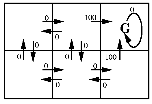
$Q(s,a)$ values are associated with $s,a$ pairs.
$V(s)$ values decrease with distance from goal.

2 Q-Learning Motivation

So we want to learn $V^{\pi^{*}} \equiv V^{*}$.
The agent could just do a lookahead search to choose the best action for each state: \[ \pi^{*}(s) = \arg \max_{a} [r(s,a) + \gamma V^{*}(\delta(s,a))] \] easy, right?
Yes, but only if we know $\delta$ and $r$.
Most often, we don't.

2.1 Q Function

Define new function very similar to $V^*$ \[ Q(s,a) \equiv r(s,a) + \gamma V^{*}(\delta(s,a)) \] If agent learns $Q$, it can choose optimal action even without knowing $\delta$ because this \[ \pi^{*}(s) = \arg \max_{a} [r(s,a) + \gamma V^{*}(\delta(s,a))] \] is the same as this \[ \pi^{*}(s) = \arg \max_{a} Q(s,a) \]
Our agent will learn $Q$.

2.2 Learning Q

We notice that $Q$ and $V^*$ are closely related, specifically: \[ V^{*}(s) = \max_{a'}Q(s,a') \]
This allows us to write $Q$ recursively as \[ Q(s_t,a_t) = r(s_t,a_t) + \gamma V^{*}(\delta(s_t,a_t))) \] \[ Q(s_t,a_t) = r(s_t,a_t) + \gamma \max_{a'}Q(s_{t+1},a') \]
Now, we let $\hat{Q}$ denote learner's current approximation to $Q$ and use the training rule \[ \hat{Q}(s,a) \leftarrow r + \gamma \max_{a'}\hat{Q}(s',a') \] where $s'$ is the state resulting from applying action $a$ in state $s$

2.3 Q-Learning Algorithm

Q-Learning Algorithm

For each $s,a$ set $\hat{Q}(s,a) = 0$.
Observe the current state $s$.
Select an action $a$ and execute it.
Receive reward $r$.
Update the table entry for $\hat{Q}(s,a)$ with \[ \hat{Q}(s,a) \leftarrow r + \gamma \max_{a'}\hat{Q}(s',a') \]
$s \leftarrow s'$ //Observe the new state.
Goto 3.

2.4 Q-Learning Example

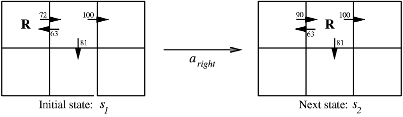
Assumes $\gamma = .9$ and the agent takes the action $a_{right}$ and gets $r = 0$.

2.5 Q-Learning Convergence

If the system is a deterministic MDP and
the immediate rewards are bounded (i.e., there is some $c$ s.t. $|r(s,a)| < c$ and
the agent visits every possible state infinitely often, then
Q-learning is proven to converge, eventually.
That is $\hat{Q}$ will eventually equal $Q$.

2.6 How to Choose an Action

Notice that the algorithm did not specify how to choose an action.
However, convergence requires that every state be visited infinitely often.
The is the classic explore vs. exploit problem! (aka, the n-armed bandit [5] problem).
A common strategy is to decide stochastically using \[ P(a_i|s) = \frac{k^{\hat{Q}(s,a_i)}}{\sum_j k^{\hat{Q}(s,a_j)}} \]

2.7 Variations

Updating after each move can make it take very long to converge if the only reward is at the end.
Instead, we can save the whole set of rewards and update at the end, in reverse order.

Another technique is to store past state-action transitions and their rewards and re-train on them periodically.
This helps when the Q values of the neighbors have changed.

2.8 Nondeterministic Rewards and Actions

The Q-learning algorithm mentioned only works for deterministic $r$ and $\delta$. Lets fix it.
First we redefine $V, Q$ by taking expected values \[ V^{\pi}(s) \equiv E[ r_{t} + \gamma r_{t+1} + \gamma^{2} r_{t+2} + \ldots \] \[ V^{\pi}(s) \equiv E \left[ \sum_{i=0}^{\infty} \gamma^{i} r_{t+i} \right] \] so that \[ Q(s,a) \equiv E[r(s,a) + \gamma V^{*}(\delta(s,a)) ] \]

2.8.1 Nondeterministic Q-Learning

We can then alter the training rule to be \[ \hat{Q}_{n}(s,a) \leftarrow (1-\alpha_{n})\hat{Q}_{n-1}(s,a) + \alpha_{n}[r+ \max_{a'}\hat{Q}_{n-1}(s',a')] \] where \[ \alpha_{n} = \frac{1}{1 + \mbox{visits}_n(s,a)} \]
Note that when $\alpha = 1$ we have the old equation. As such, all we are doing is making revisions to $\hat{Q}$ more gradual.
We can still prove convergence of $\hat{Q}$ to $Q$.

3 Temporal Difference Learning

$Q$ learning acts to reduce the difference between successive $Q$ estimates, in one-step time differences: \[ Q^{(1)}(s_t,a_t) \equiv r_t + \gamma \max_{a} \hat{Q}(s_{t+1},a) \] So, why not use two steps? \[ Q^{(2)}(s_t,a_t) \equiv r_t + \gamma r_{t+1} + \gamma^2 \max_{a} \hat{Q}(s_{t+2},a) \] Or $n$ steps? \[ Q^{(n)}(s_t,a_t) \equiv r_t + \gamma r_{t+1} + \cdots + \gamma^{(n-1)}r_{t+n-1} + \gamma^n \max_{a}\hat{Q}(s_{t+n},a) \]
We can blend all these by letting $\lambda$ be the number of steps we wish to use: \[Q^{\lambda}(s_{t},a_{t}) \equiv (1- \lambda) \left[ Q^{(1)}(s_t,a_t) + \lambda Q^{(2)}(s_t,a_t) + \lambda^2 Q^{(3)}(s_t,a_t) + \cdots \right] \]

3.1 Temporal Difference

We can then rewrite it as a recursive function \[ Q^{\lambda}(s_{t},a_{t}) = r_{t} + \gamma [ (1 - \lambda) \max_{a}\hat{Q}(s_{t},a_{t})+ \lambda Q^{\lambda}(s_{t+1},a_{t+1})] \]
The TD($\lambda$) [6] algorithm (by Sutton [7]) uses this training rule.
TD($\lambda$) sometimes converges faster than Q-learning.
TD-Gammon uses it.

4 Generalization from Examples

Often there are way too many states to build a table,
or the state is not completely visible.
We can fix this by replacing $\hat{Q}$ with a neural net or other generalizer.
1. For example, encode $s,a$ as the network inputs and train it to output the target values of $\hat{Q}$ given by the training rules.
2. Or, train a separate network for each action, using the state as input and $\hat{Q}$ as output.
3. Or, train one network with the state as input but with one $\hat{Q}$ output for each action.
TD-Gammon used neural nets and Backpropagation.