Instance Based Learning

So far, we have considered algorithms that search for a hypothesis that matches all the training data.
Instance-based algorithms simply store the presented data.
When a new query arrives they try to match it with similar instances and use them to classify.
For example, given 10 fossil remains, each of a different species, I might try to classify a new fossil remain by finding the one that looks most similar.

2 k-Nearest Neighbor Learning

Assume all instances correspond to point in n-dimensional space.
Store all training examples $\langle x_i, f(x_i) \rangle$.
Given that an instance $x$ is described by its feature vector \[ \langle a_1(x),a_2(x)\ldots a_n(x)\rangle \] we define the distance as \[ d(x_i,x_j) \equiv \sqrt{\sum_{r=1}^{n}(a_r(x_i)-a_r(x_j))^2} \]
Nearest Neighbor: To classify a new instance $x_q$ first locate nearest training example $x_n$, then estimate $\hat{f}(x_q) \leftarrow f(x_n)$
$k$-Nearest Neighbor Take a vote among the $k$ nearest neighbors, if discrete $f$. If continuous $f$ then take mean \[\hat{f}(x_{q}) \leftarrow \frac{\sum_{i=1}^{k}f(x_{i})}{k}\]

2.1 When to Use K-Nearest

When the instances are points in Euclidean space.
When there are few attributes (why?)
When there is a lot of training data
Advantages
- Training is very fast
- Learn complex target functions
- Don't lose information
Disadvantages
- Slow at query time
- Easily fooled by irrelevant attributes

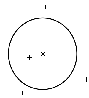
2.2 Voronoi Diagram

A Voronoi diagram

The hypothesis space implicitly considered by the 1-Nearest neighbor algorithm is given by a Voronoi diagram.
What does the picture look like for the k-Nearest?

2.3 Behavior in the Limit

Consider $p(x)$ defines probability that instance $x$ will be labeled 1 (positive) versus 0 (negative).
Nearest neighbor: As number of training examples goes to $\infty$, approaches Gibbs Algorithm (i.e., with probability $p(x)$ predict 1, else 0)
k-Nearest neighbor: As number of training examples goes to $\infty$ and $k$ gets large, approaches Bayes optimal (i.e., if $p(x)>.5$ then predict 1, else 0)

2.4 Distance-Weighted kNN

We might want to weight the nearer neighbors more heavily: \[ \hat{f}(x_{q}) \leftarrow \frac{\sum_{i=1}^{k} w_{i} f(x_{i})}{\sum_{i=1}^{k} w_{i}} \] where \[ w_{i} \equiv \frac{1}{d(x_{q}, x_{i})^{2}} \] and $d(x_{q}, x_{i})$ is distance between $x_{q}$ and $x_{i}$.
Using this function it makes sense to use all examples instead of just $k$.
If all training examples are used we call the algorithm a global method. If only the nearest are use then its a local method.

2.5 Curse of Dimensionality

The inductive bias of the kNN corresponds to the assumption that the classification of an instance will be most similar to other instances that are nearby in Euclidean distance.
This means that all attributes are used.
A problem: 20 attributes but only 2 are relevant to the target function.
This is the curse of dimensionality
One approach is to weigh each attribute differently.
- Stretch $j$th axis by weight $z_j$, where $z_1, \ldots, z_n$ chosen to minimize prediction error.
- Use cross-validation to automatically choose weights $z_1, \ldots, z_n$.
- Note setting $z_j$ to zero eliminates this dimension altogether (another approach).

3 Notation

Before we go on, we need some definitions:
Regression means approximating a real-valued target function.
Residual is the error $\hat{f}(x) - f(x)$ in approximating the target function.
Kernel function is the function of distance that is used to determine the weight of each training example. That is, $K$ where \[ w_i = K(d(x_i, x_q))\]

4 Locally Weighted Regression

The kNN approximates the target function for a single query point.
Locally Weighted Regression is a generalization of that approach. It constructs an explicit approximation to $f$ over a local region surrounding $x_q$.
We can try to form an explicit approximation $\hat{f}(x)$ for the region surrounding $x_q$.
Assume that \[ \hat{f}(x) \equiv w_0 + w_1 a_1(x) + \cdots + w_n a_n(x) \]

We can minimize the squared error over $k$ nearest neighbors \[E_{1}(x_q) \equiv \frac{1}{2} \sum_{x \in k nearest nbrs of x_q} (f(x) - \hat{f}(x))^2 \]
We can minimize the instance-weighted squared error over all neighbors \[E_{2}(x_q) \equiv \frac{1}{2} \sum_{x \in D} (f(x) - \hat{f}(x))^2 K(d(x_{q}, x)) \]
Or, we can combine these two \[E_{2}(x_q) \equiv \frac{1}{2} \sum_{x \in k nearest nbrs of x_q} (f(x) - \hat{f}(x))^2 K(d(x_{q}, x)) \]

Eq. 2 two is more aesthetically pleasing but Eq. 3 is a good approximation with costs that depend on $k$.

4.1 Local Regression Descent

If we choose Eq. 3, we have to re-derive a gradient descent rule using the same arguments as for neural nets.
As such, we can adjust the weights of $\hat{f}(x)$ with \[ \Delta w_i \equiv \eta \sum_{x\in k nearest nbrs of x_q} K(d(x_q,x))(f(x)-\hat{f}(x))a_j(x) \]
This equation will do gradient descent on the weights of $\hat{f}(x)$ so as to minimize its error against $f(x)$.
There are many other much more efficient methods to fit linear functions to a set of fixed training examples (see book for references).
Locally Weighted Regression often uses linear or quadratic functions because more complex functions are too hard to fit and only provide marginal benefits, at best.

5 Radial Basis Functions

Instead of using a linear function, we try to learn a function of the form \[ \hat{f}(x) = w_0 + \sum_{u=1}^{k} w_u K_u(d(x_u,x)) \] where each $x_u$ is an instance from $X$ where the kernel function $K_u(d(x_u,x))$ is defined so that it decreases as the distance $d(x_u,x)$ increases.
$k$ is a user-defined constant that specifies the number of kernel functions to be included.
Note that, even thought $\hat{f}(x)$ is a global approx to $f(x)$, the contribution from each of the $K_u$ terms is localized to a region near $x_u$.
It is common to choose $K$ to be a Gaussian centered around $x_u$ \[ K_u(d(x_u,x)) = e^{\frac{d^2(x_{u},x)}{2\sigma_u^2}} \]
It has been shown that this $\hat{f}(x)$ can approximate any function with arbitrarily small error, given enough $k$ and given that each $\sigma^2$ can be separately specified.

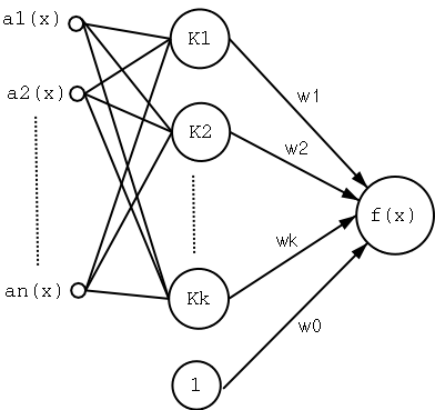
5.1 Radial Basis Function Networks

We can view the new $\hat{f}(x)$ as a two-layer network were the first layer computes the various $K$ and the second does the linear combination of them.
The network can be trained in two stages:

The number $k$ of hidden units is determined and each unit $u$ is defined by choosing the values of $x_u$ and $\sigma_u^2$ that define its kernel function $K_u(d(x_u,x))$ (e.g., with EM).
The weights $w_u$ are trained to maximize the fit of the network to the data using the global squared error criterion.

Since the $K_u$ are fixed for the second step it can be trained with efficient linear function fit methods.

6 Case-Based Reasoning

In CBR the instances are represented by rich symbolic descriptions, not by points in space.
Useful when we can't represent instances as points in space.

The representations often use symbolic logic representations. The examples consist of a series of facts

((user-complaint error53-on-shutdown)
 (cpu-model PowerPC)
 (operating-system Windows)
 (network-connection PCIA)
 (memory 48meg)
 (installed-applications Excel Netscape VirusScan)
 (disk 1gig)
 (likely-cause ???))

6.1 CADET

The CADET [3] system was designed to assist in the design of mechanical devices.
It stores 75 examples of mechanical devises.
Each training example consists of a pair [Structure, Function].
A query provides the functions and asks for any structure that has a similar function.
The structure is a diagram of the device. The function is a high-level description of what it does.

6.2 CADET Answers

CADET first tries to find an exact match.
If no match is found then try to match various subgraphs of the desired functional specification (that is, match parts).
If multiple cases match different subgraphs then maybe the entire query can be pieced together.
If still no match, then elaborate existing examples in order to create graphs that might match. For example \[A \rightarrow B\] becomes \[A \rightarrow x \rightarrow B\]

6.3 CADET vs. k-Nearest

CADET represents instances with rich symbolic descriptions so it needs a new similarity metric (e.g., size of largest shared subgraph).
Both can use multiple examples in classification, but they combine them in different ways. CADET must have special rules for combining.
CBR, in general, shows a tight coupling between case retrieval, knowledge-based reasoning, and problem solving.
CBR is useful for simple matching of queries such as help-desk questions.

6.4 CBR Summary

CBR continues to be an area of research.
There are many successful commercial applications. It is useful for help-desk-type situations where the same few problems keep cropping up (only a few points on H).
More info on the CBR web [4].

7 Lazy and Eager Learning

Instance-based methods are also known as lazy learning because they do not generalize until needed.
All the other learning methods we have seen (and even radial basis function networks) are eager learning methods because they generalize before seeing the query.
The eager learner must create a global approximation.
The lazy learner can create many local approximations.
If they both use the same $H$ then, in effect, the lazy can represent more complex function.
For example, if $H$ consists of linear function then a lazy learner can construct what amounts to a non-linear global function.